Turns out WWII was pretty complicated.
History, and historians, are full of “what ifs.” What if the typhoons of 1274 and 1281 hadn’t stopped the Mongols from invading Japan? What if Oliver Cromwell had gone through with his plans to emigrate to America? What if Chernobyl Unit 4 hadn’t exploded?
Here’s another one for you: What if we could use machine learning to answer these what-ifs?
First of all, let’s get the spoiler alert out of the way: no, we can’t, not in any meaningful way. There’s far too much essential data for any model to process, and most of that is lost forever in time. More importantly, trying to predict “alternate histories” is basically a supervised learning problem for causality, but unless we can travel among parallel timelines, we don’t have true labels to train on.
It’s tempting to apply Judea Pearl’s do-calculus and/or structural equation modeling to the problem, but the problem there is similar: we don’t have many concrete, provable instances of causation in history, and historical causation itself can be extremely complex. For example, there’s a debatable though not-unreasonable theory that the Fukushima disaster in 2011 led to the 2022 invasion of Ukraine. It’s hard to imagine a model complex enough to predict a causal chain like that.
What we can do, however, is build a model around the history we do know, then do a bit of data manipulation to explore counterfactuals - as long as we’re scrupulous about not asserting causation. To do this, we can use GNNs, along with a few tricks to help us ask those “What If?” questions.
Living in Infamy
For this project, I picked World War II as the era to model, for sevaral reasons:
- The war happened in somewhat recent times, so the “fog of history” is still fairly thin.
- The was isn’t so recent that propaganda, misinformation and internet debates would drown out useful signals.
- World War II was a complex and enormous event, so there are many data points to train on.
Before continuing, it’s worth reflecting that World War II was about people, not data. Countless millions of people were killed or injured, displaced or bereaved. As kids, it’s fine to play with plastic tanks and model fighters, but as adult data scientists and AI engineers, we should never forget where the data come from and what they mean, lest we trivialize the things we’re trying to understand.
Choosing the Data Format
History moves forward in a straight line, which might suggest a time-series for storing the events of WWII or any given historical era. But it’s easy to see how this doesn’t make much sense. On May 19th 1941, the Viet Minh was formed, and the next day, the Battle of Crete began. The subsequence of those two events probably has little to do with how closely they were related. Sure, we could concoct some complex embeddings, attention mechanisms and loss functions to account for non-chronological factors, but before long we’d end up with something that no longer looks like a time series.
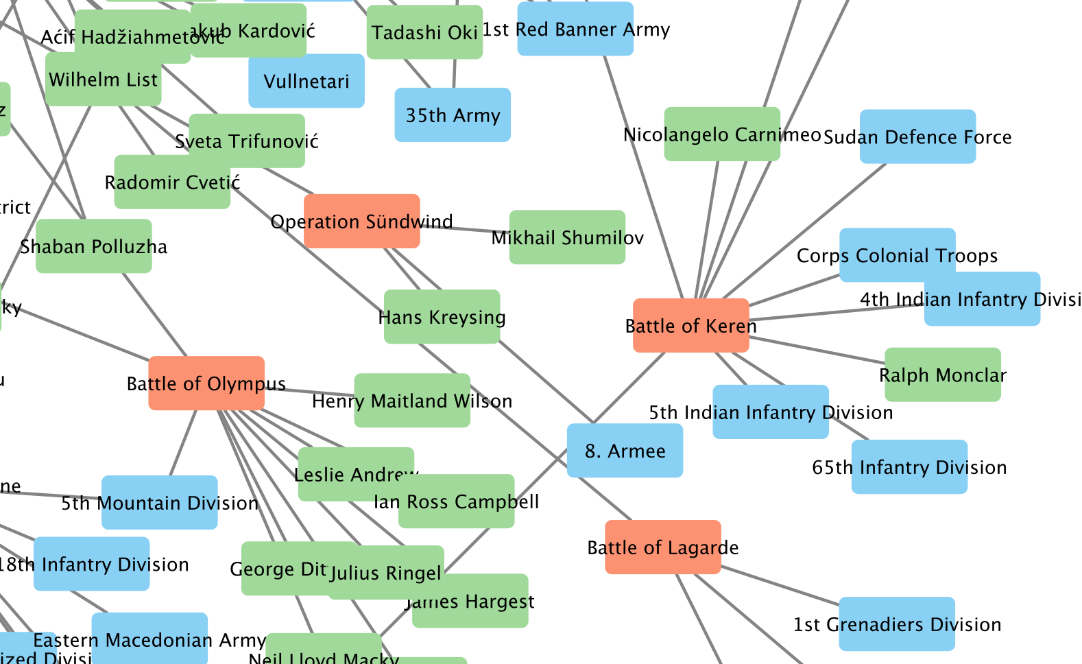
In fact, what we’d probably end up with is what I used: a graph. Since I chose Wikipedia as my primary data source, building a graph is a natural step, since Wikipedia itself is basically “graph shaped.” I decided to build a heterogeneous graph, since the events and actors in the war are too. For starters, I chose three node types:
- battles
- military units
- commanders
I picked these not just because they were the most immediately available “object types” in Wikipedia WWII pages, but because using them would allow me to ask counterfactual questions by changing or ablating nodes. For example, what if Chester Nimitz hadn’t been at Midway? What if the Battle of the North Cape simply hadn’t happened?
Mining Wikipedia
Once I chose the graph type, it was time to fill it with data. I build a pipeline to traverse Wikipedia, downloading the Wikitext from articles that belonged to several “Battle of WWII” categories, and following links to supporting articles. At first I tried building a parser for the Infoboxes that nearly every battle article has, like this one:
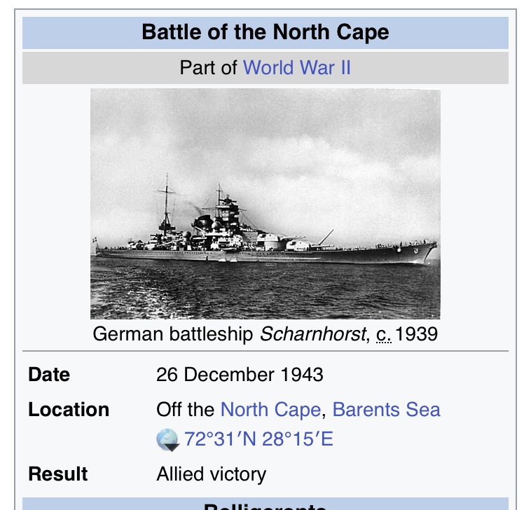
Infobox: It’s Info, In a Box™
Seemed like a reasonable approach - right there, in handy little sections, was all the data I needed. But as it turns out, even these Infoboxes suffered from a lot of format variation. It was a reminder to me that Wikipedia is a nearly all-volunteer organization, written and edited by human beings, and nobody’s getting fired for coloring outside the lines a bit. I kept having to handle more and more edge cases, until I finally gave in to my lazier instincts: let an LLM parse it, and emit standardized JSON for each battle.
{
  "event_name": "Battle of the North Cape",
  "event_type": "battle",
  "source_url": "https://en.wikipedia.org/wiki/Battle_Of_The_North_Cape",
  "date": "1943-12-26",
  "date_precision": "day",
  "location": {
    "name": "Off the North Cape, Barents Sea",
    "latitude": 72.51666666666667,
    "longitude": 28.25
  },
  "belligerents": {
    "1": {
      "countries": [
        {
          "name": "United Kingdom",
          "commanders": [
            "Bruce Fraser"
          ],
Some of the battles didn’t have exact geographic data (which I would need for training), so I used both Wikidata and Nominatim as fallbacks for those, and got pretty close to 99% coverage on geodata. Some articles covered battles so massive that they had separate “order of battle” pages - basically, a thorough listing of the units that participated, so I downloaded and processed those too.
The end result was a heterogenous grapy (NetworkX MultiDiGraph) of the 1000 or so most significant battles of WWII, with commanders and military units as nodes with directed edges to battle nodes. This also means three edge types: COMMANDED_IN, FOUGHT_IN, HAS_SUBUNIT
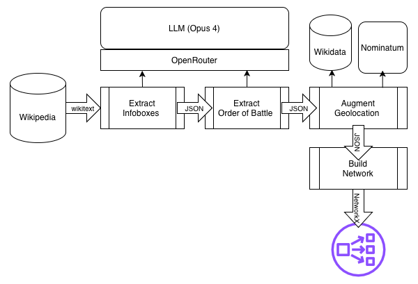
The Wikipedia-to-NetworkX pipeline.
Building the Model
The goal at this point was battle outcome prediction — a 3-class node classification problem predicting which side won each battle (side_1, side_2 or unknown).
During dataset preparation, COMMANDED_IN and FOUGHT_IN edges are split by belligerent side (e.g., commanded_in_side1, commanded_in_side2) so that HGTConv can distinguish which side a commander or unit fought on without needing edge
attributes.
Feature Engineering
Each node type gets its own feature vector:
- Battle (~86 scalar features, optionally +384-dim sentence embedding): normalized start date, log-normalized duration, date precision (one-hot), lat/lon, outcome (one-hot), winning_side (one-hot), nations (multi-hot). Outcome text is
stripped from descriptions to prevent leakage. - Commander (~73 features): nation multi-hot, has_nation flag, in/out degree, battle count - Unit (~79 features): unit type one-hot (7 categories), nation one-hot, has_nation flag, subunit in-degree, battle count
Then comes the part where we do our train, evaluation, and test splits. The trick here is to sort the battles chronologically, so we don’t have information “leaking from the future.” (That part sounds a lot more sci-fi than it actually is.) Then I masked the outcomes, so that the model wouldn’t know the winning side for battles beyond the time horizon we were training on.
I experimented with two GNN types:
- HGT (Heterogeneous Graph Transformer)
- Per-type linear input projections to a shared hidden dimension (default 128)
- 2 stacked HGTConv layers with 4-head attention
- Residual connections + LayerNorm + ReLU + dropout (0.3) after each layer
- Battle-only MLP classification head: hidden → hidden/2 → ReLU → dropout → num_classes
- GraphSAGE
- Same per-type input projections
- Single HeteroConv layer wrapping SAGEConv per edge type (aggregation = sum)
- Same residual + LayerNorm + ReLU + dropout pattern
- Same MLP classification head
The key difference: HGT uses multi-head attention across 2 layers to learn type-aware attention weights over neighbors, while GraphSAGE uses a single layer of mean/sum neighborhood aggregation per edge type — simpler and more inductive but less expressive.
I optimized with Adam (lr=0.001, weight_decay=1e-4), and picked cross-entropy loss with inverse-frequency class weights to handle class imbalance (so, basically focal loss, but without the “penalty” on easy cases).
All runs were tracked by Weights and Biases.
Initial Results
Eh… not great. The HGT yielded a macro F1 of 0.366, so, not really higher than chance. The confusion matrix makes it a little more clear where the model is stumbling:
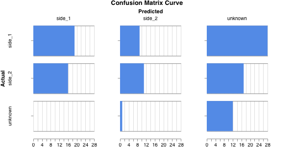
Testing the HGT ability to predict battle outcomes.
For GraphSAGE, the macro F1 was 0.469, so significantly better, and the confusion matrix:
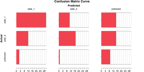
Testing the HGT ability to predict battle outcomes.
HGT was almost certainly overfitting; it does better with significantly more data (and specifically, more edges), and that was made worse with the temporal masking we used. But, both model types underperformed expectations. In fact, I trained a simple MLP model on just the node attributes, and got a macro F1 above .5, higher than either one. The graph connections were arguably confusing the model, not helping it. With such unimpressive results, I didn’t bother trying to perturb the data and test counterfactuals, e.g. removing Admiral Nimitz from Midway to see what happens. No sense trying to predict alternate histories when you don’t even have a decent model of this one.
What Next?
It’s tempting to wonder if GraphSAGE (or even HGT) might benefit from hyperparameter sweeps, which Weights and Biases is very handy for, and which I didn’t bother with. Ultimately, though, this seems more like a feature engineering problem, and a big one.
Also, this might call for a more appropriate graph type, specifically, temporal graph networks, or applying neural causal models for counterfactual identification. So, this is a work in progress… much like history itself.